Regression with Interaction Terms - How Centering Predictors influences Main Effects'
Centering predictors in a regression model with only main effects has no influence on the main effects. In contrast, in a regression model including interaction terms centering predictors does have an influence on the main effects. After getting confused by this, I read this nice paper by Afshartous & Preston (2011) on the topic and played around with the examples in R. I summarize the resulting notes and code snippets in this blogpost.
We give an explanation on two levels:
- By illustrating the issue with the simplest possible example
- By showing in general how main effects are a function of the constants (e.g. means) that are substracted from predictor variables
Explanation 1: Simplest example
The simplest possible example to illustrate the issue is a regression model in which variable $Y$ is a linear function of variables $X_1$, $X_2$, and their product $X_1X_2$
\[Y = \beta_0 + \beta_1 X_1 + \beta_2 X_2 + \beta_3 X_1X_2 + \epsilon,\]where we set $\beta_0 = 1, \beta_1 = 0.3, \beta_2 = 0.2, \beta_3 = 0.2$, and $\epsilon \sim N(0, \sigma^2)$ is Gaussian distribution with mean zero and variance $\sigma^2$. We define the predictors $X_1, X_2$ as Gaussians with means $\mu_{X_1} = \mu_{X_2} = 1$ and $\sigma_{X_1}^{2}=\sigma_{X_2}^{2}=1$. This code samples $n = 10000$ observations from this model:
n <- 10000
b0 <- 1; b1 <- .3; b2 <- .2; b3 <- .2
set.seed(1)
x1 <- rnorm(n, mean = 1, sd = 1)
x2 <- rnorm(n, mean = 1, sd = 1)
y <- b0 + b1 * x1 + b2 * x2 + b3 * x1 * x2 + rnorm(n, mean = 0, sd = 1)
Regression models with main effects
We first verify that centering variables indeed does not affect the main effects. To do so, we first fit the linear regression with only main effects with uncentered predictors
lm(y ~ x1 + x2)##
## Call:
## lm(formula = y ~ x1 + x2)
##
## Coefficients:
## (Intercept) x1 x2
## 0.8088 0.4983 0.4015and then with mean centered predictors
x1_c <- x1 - mean(x1) # center predictors
x2_c <- x2 - mean(x2)
lm(y ~ x1_c + x2_c)
##
## Call:
## lm(formula = y ~ x1_c + x2_c)
##
## Coefficients:
## (Intercept) x1_c x2_c
## 1.7036 0.4983 0.4015The parameter estimates of the regression with uncentered predictors are $\hat\beta_1 \approx 0.50$ and $\hat\beta_2 \approx 0.40$. The estimates of the regression with centered predictors are $\hat\beta_1^\ast \approx 0.50$ and $\hat\beta_2^\ast \approx 0.40$ (we denote estimates from regressions with centered predictors with an asterisk). And indeed, $\hat\beta_1 = \hat\beta_1^\ast$ and $\hat\beta_2 = \hat\beta_2^\ast$.
Regression models with main effects + interaction
We include the interaction term and show that centering the predictors now does does affect the main effects. We first fit the regression model without centering
lm(y ~ x1 * x2)##
## Call:
## lm(formula = y ~ x1 * x2)
##
## Coefficients:
## (Intercept) x1 x2 x1:x2
## 1.0183 0.2883 0.1898 0.2111and then with centering
lm(y ~ x1_c * x2_c)##
## Call:
## lm(formula = y ~ x1_c * x2_c)
##
## Coefficients:
## (Intercept) x1_c x2_c x1_c:x2_c
## 1.7026 0.4984 0.3995 0.2111We see that $\hat\beta_1 \approx 0.29$ and $\hat\beta_2 \approx 0.19$ and $\hat\beta_1^\ast \approx 0.50$ and $\hat\beta_2^\ast \approx 0.40$. While the two models have different parameters, they are statistically equivalent. Here this means that expected values of both models are the same. In empirical terms this means that their coefficient of determination $R^2$ is the same. The reader will be able to verify this in Explanation 2 below.
We make two observations:
- In the model with interaction terms, the main effects differ between the regressions with/without centering of predictors
- When centering predictors, the main effects are the same in the model with/without the interaction term (up to some numerical inaccuracy)
Why does centering influence main effects in the presence of an interaction term?
The reason is that in the model with the interaction term, the parameter $\beta_1$ (uncentered predictors) is the main effect of $X_1$ on $Y$ if $X_2 = 0$, and the parameter $\beta_1^\ast$ (centered predictors) is the main effect of $X_1$ on $Y$ if $X_2 = \mu_{X_2}$. This means that $\beta_1$ and $\beta_1^\ast$ are modeling different effects in the data. Here is a more detailed explanation:
Rewriting the model equation in the following way
\[\begin{aligned} \mathbb{E}[Y] &= \beta_0 + \beta_1 X_1 + \beta_2 X_2 + \beta_3 X_1X_2 \\ &= \beta_0 + (\beta_1 + \beta_3 X_2) X_1 + \beta_2 X_2 \end{aligned}\]shows that in the model with interaction term, the effect of $X_1$ on $Y$ is equal to $(\beta_1 + \beta_3 X_2)$ and therefore a function of $X_2$. What does the parameter $\beta_1$ model here? It models the effect of $X_1$ on $Y$ when $X_2 = 0$. Similarly we could rewrite the effect of $X_1$ on $Y$ as a function of $X_2$.
Now let $X_1^c = X_1 - \mu_{X_1}$ and $X_2^c = X_2 - \mu_{X_2}$ be the centered predictors. We get the same model equations, now with the parameters estimated using the centered predictors $X_1^c, X_2^c$:
\[\begin{aligned} \mathbb{E}[Y] &= \beta_0^\ast + \beta_1^\ast X_1^c + \beta_2^\ast X_2^c + \beta_3^\ast X_1^c X_2^c \\ &= \beta_0^\ast + (\beta_1^\ast + \beta_3^\ast X_2^c) X_1^c + \beta_2^\ast X_2^c \\ \end{aligned}\]Again we focus on the effect $(\beta_1^\ast + \beta_3^\ast X_2^c)$ of $X_1^c$ on $Y$. What does the the parameter $\beta_1^\ast$ model here? It models the main effect of $X_1^c$ on $Y$ when $X_2^c = \mu_{X_2^c} = 0$. What remained the same is that $\beta_1^\ast$ is the main effect of $X_1^c$ on $Y$ when $X_2^c = 0$. But what is new is that $\mu_{X_2^c} = 0$.
To summarize, in the uncentered case $\beta_i$ is the main effect when the predictor variable $X_i$ is equal to zero; and in the centered case, $\beta_i^\ast$ is the main effect when the predictor variable $X_i$ is equal to its mean. Clearly, $\beta_i$ and $\beta_i^\ast$ model different effects in the data and it is therefore not surprising that the two regressions give us very different estimates.
Centering $\rightarrow$ interpretation of $\beta$ remains the same when adding interaction
Our second observation above was that the estimates of main effects are the same with/without interaction term when centering the predictor variables. This is because in the models without interaction term (centered or uncentered predictors) the interpretation of $\beta_1$ is the same as in the model with interaction term and centered predictors.
More precisely, in the regression model with only main effects, $\beta_1$ is the main effect of $X_1$ on $Y$ averaged over all values of $X_2$, which is the same as the main effect of $X_1$ on $Y$ for $X_2 = \mu_{X_2}$. This means that if we center predictors, $\beta_1$ models the same effect in the data in a model with/without interaction term. This is an attractive property to have when one is interested in comparing models with/without interaction term.
Explanation 2: Main effects as functions of added constants
Substracting the mean from predictors is a special case of adding constants to predictors. Here we first show numerically what happens to each regression parameter when adding constants to predictors. Then we show analytically how each parameter is a function of its value in the original regression model (no constant added) and the added constants.
Why are we doing this? We are doing this to develop a more general understanding of what happens when adding constants to predictors. It also puts the above example in a more general context, since we can consider it as a special case of the following analysis.
Numerical experiment I: Only main effects
We first fit a series of regression models with only main effects. In each of them we add a different constant to the predictors. We do this verify that our claim that centering predictors does not change main effects extends to the more general situation of adding constants to predictors.
We first define a sequence of constant values we add to the predictors and create storage for parameter estimates:
n <- 25
c_sequence <- seq(-1.5, 1.5, length = n)

A <- as.data.frame(matrix(NA, ncol=5, nrow=n))
colnames(A) <- c("b0", "b1", "b2", "b3", "R2")
We now fit 25 regression models, and in each of them we add a constant c to both predictors, taken from the sequence c_sequence:
for(i in 1:25) {

  c <- c_sequence[i]
  x1_c <- x1 + c
  x2_c <- x2 + c

  lm_obj <- lm(y ~ x1_c + x2_c) # Fit model
  A$b0[i] <- lm_obj$coefficients[1]
  A$b1[i] <- lm_obj$coefficients[2]
  A$b2[i] <- lm_obj$coefficients[3]

  yhat <- predict(lm_obj)
  A$R2[i] <- 1 - var(yhat - y) / var(y) # Compute R2

}
Remark: in Explanation 1 we said that the coefficient of determination $R^2$ does not change when adding constants to the predictors. We invite the reader to verify this by inspecting A$R2.
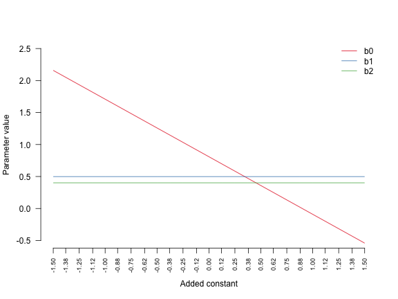
We plot all parameters $\beta_0, \beta_1, \beta_2$ as a function of c:
library(RColorBrewer)
cols <- brewer.pal(4, "Set1") # Select nice colors

plot.new()
plot.window(xlim=range(c_sequence), ylim=c(-.5, 2.5))
axis(1, round(c_sequence, 2), cex.axis=0.75, las=2)
axis(2, c(-.5, 0, .5, 1, 1.5, 2, 2.5), las=2)
lines(c_sequence, A$b0, col = cols[1])
lines(c_sequence, A$b1, col = cols[2])
lines(c_sequence, A$b2, col = cols[3])
legend("topright", c("b0", "b1", "b2"),
       col = cols[1:3], lty = rep(1,3), bty = "n")
title(xlab = "Added constant")
title(ylab = "Parameter value")
We see that the intercept changes as a function of c. The model at c = 0 corresponds to the very first model we fitted above. And the model at c = -1 corresponds to the model fitted with centered predictors. But the key observation is that the main effects $\beta_1, \beta_2$ do not change. A proof of this and an exact expression for the intercept will fall out of our analysis of the model with interaction term in the last section of this blogpost.
Numerical experiment II: main effects + interaction term
Next we show that this is different when adding the interaction term. We use the same sequence of c as above and fit regression models with interaction term:
for(i in 1:25) {

  c <- c_sequence[i]
  x1_c <- x1 + c
  x2_c <- x2 + c

  lm_obj <- lm(y ~ x1_c * x2_c) # Fit model
  A$b0[i] <- lm_obj$coefficients[1]
  A$b1[i] <- lm_obj$coefficients[2]
  A$b2[i] <- lm_obj$coefficients[3]
  A$b3[i] <- lm_obj$coefficients[4]

  yhat <- predict(lm_obj, data = c(y, x1_c, x2_c))
  A$R2[i] <- 1 - var(yhat - y) / var(y) # Compute R2

}
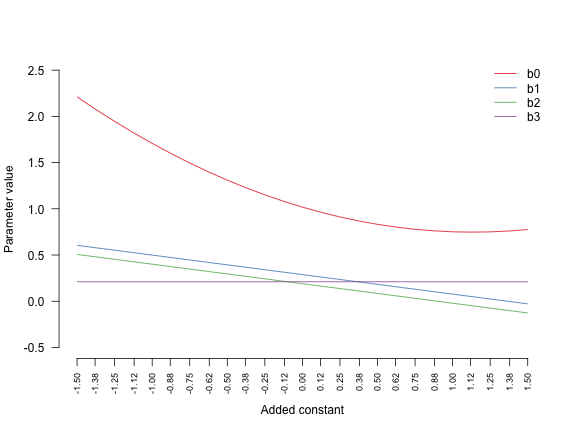
And again we plot all parameters $\beta_0, \beta_1, \beta_2, \beta_3$ as a function of c:
plot.new()
plot.window(xlim=range(c_sequence), ylim=c(-.5, 2.5))
axis(1, round(c_sequence, 2), cex.axis=0.75, las=2)
axis(2, c(-.5, 0, .5, 1, 1.5, 2, 2.5), las=2)
lines(c_sequence, A$b0, col = cols[1])
lines(c_sequence, A$b1, col = cols[2])
lines(c_sequence, A$b2, col = cols[3])
lines(c_sequence, A$b3, col = cols[4])
legend("topright", c("b0", "b1", "b2", "b3"),
       col = cols[1:4], lty = rep(1,3), bty = "n")
title(xlab = "Added constant")
title(ylab = "Parameter value")
This time both the intercept $\beta_0$ and the main effects $\beta_1, \beta_2$ are a function of c, while the interaction effect $\beta_3$ is constant. At this point the best explanation is simply to go through the algebra, which explains these results exactly. We do this in the next section.
Deriving function for all effects
We plug in the definition of centering in the population regression model we introduced at the very beginning of this blogpost. This gives us every parameter as a function of two things: (1) the parameters in the original model and (b) the added constant. Above we added the same constant to both predictors. Here we consider the general case where the constants can differ.
Our original (unaltered) model is given by:
\[\begin{aligned} \mathbb{E}[Y] &= \beta_0 + \beta_1 X_1 + \beta_2 X_2 + \beta_3 X_1X_2 \end{aligned}\]Now we plug in the predictors with added constants $c_1, c_2$, multiply out, and rearrange:
\[\begin{aligned} \mathbb{E}[Y] &= \beta_0^\ast + \beta_1^\ast (X_1 + c_1) + \beta_2 (X_2 + c_2) + \beta_3^\ast (X_1 + c_1) (X_2 + c_2) \\ & = \beta_0^\ast + \beta_1^\ast X_1 + \beta_1^\ast c_1 + \beta_2^\ast X_2 + \beta_2^\ast c_2 + \beta_3^\ast X_1X_2 + \beta_3^\ast X_1 c_2 + \beta_3^\ast c_1X_2 + \beta_3^\ast c_1c_2 \\ &= (\beta_0^\ast + \beta_1^\ast c_1 + \beta_2^* c_2 + \beta_3^\ast c_1c_2) + (\beta_1^\ast + \beta_3^\ast c_2)X_1 + (\beta_2^\ast + \beta_3^\ast c_1)X_2 + \beta_3^\ast X_1X_2 \end{aligned}\]Now if we equate the respective interecept and slope terms we get:
\[\beta_0 = \beta_0^\ast + \beta_1^\ast c_1 + \beta_2^\ast c_2 + \beta_3^\ast c_1c_2\] \[\beta_1 = \beta_1^\ast + \beta_3^\ast c_2\] \[\beta_2 = \beta_2^\ast + \beta_3^\ast c_1\]and
\[\beta_3 = \beta_3^\ast\]Now we solve for the parameters $\beta_0^\ast, \beta_1^\ast, \beta_2^\ast, \beta_3^\ast$ from the models with constants added to the predictors.
Because we know $\beta_3 = \beta_3^\ast$ we can write $\beta_2 = \beta_2^\ast + \beta_3 c_1$ and can solve
\[\beta_2^\ast = \beta_2 - \beta_3 c_1\]The same goes for $\beta_1^\ast$ so we have
\[\beta_1^\ast = \beta_1 - \beta_3 c_2\]Finally, to obtain a formula for $\beta_0^\ast$ we plug the just obtained expressions for $\beta_1^\ast$, $\beta_2^\ast$ and $\beta_3^\ast$ into
\[\beta_0 = \beta_0^\ast + \beta_1^\ast c_1 + \beta_2^\ast c_2 + \beta_3^\ast c_1c_2\]and get
\[\begin{aligned} \beta_0 &= \beta_0^\ast + (\beta_1 - \beta_3 c_2)c_1 + (\beta_2 - \beta_3 c_1)c_2 + \beta_3 c_1c_2 \\ &= \beta_0^\ast + \beta_1 c_1 - \beta_3 c_2 c_1 + \beta_2 c_2 - \beta_3 c_2 c_1 + \beta_3 c_1c_2 \\ &= \beta_0^\ast + \beta_1 c_1 + \beta_2 c_2 - \beta_3 c_1c_2 \end{aligned}\]and can solve for $\beta_0^\ast$:
\[\beta_0^\ast = \beta_0 - \beta_1 c_1 - \beta_2 c_2 + \beta_3 c_1c_2\]Let’s check whether those fomulas predict the parameter changes as a function of c in the numerical experiment above.
lm_obj <- lm(y ~ x1 * x2) # Reference model (no constant added)
b0 <- lm_obj$coefficients[1]
b1 <- lm_obj$coefficients[2]
b2 <- lm_obj$coefficients[3]
b3 <- lm_obj$coefficients[4]

B <- A # Storage for predicted parameters

for(i in 1:25) {

c <- c_sequence[i]

B$b0[i] <- b0 - b1*c - b2*c + b3*c*c
B$b1[i] <- b1 - b3*c
B$b2[i] <- b2 - b3*c
B$b3[i] <- b3

}
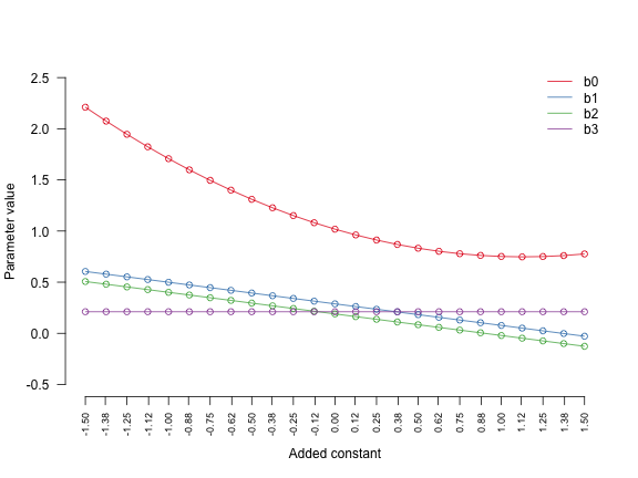
We plot the computed parameters by the derived expressions as points on the empirical results from the numerical experiments above
plot.new()
plot.window(xlim=range(c_sequence), ylim=c(-.5, 2.5))
axis(1, round(c_sequence, 2), cex.axis=0.75, las=2)
axis(2, c(-.5, 0, .5, 1, 1.5, 2, 2.5), las=2)
lines(c_sequence, A$b0, col = cols[1])
lines(c_sequence, A$b1, col = cols[2])
lines(c_sequence, A$b2, col = cols[3])
lines(c_sequence, A$b3, col = cols[4])
legend("topright", c("b0", "b1", "b2", "b3"),
col = cols[1:4], lty = rep(1,3), bty = "n")

# Plot predictions
points(c_sequence, B$b0, col = cols[1])
points(c_sequence, B$b1, col = cols[2])
points(c_sequence, B$b2, col = cols[3])
points(c_sequence, B$b3, col = cols[4])
title(xlab = "Added constant")
title(ylab = "Parameter value")
and they match the numerical results exactly.
We see that the derived expressions explain exactly how parameters change as a function of the parameters of the reference model and the added constants.
If we set $\beta_3 = 0$, we get the same derivation for the regression model without interaction term. We find that $\beta_1^* = \beta_1$, $\beta_2^* = \beta_2$, and $\beta_0^* = \beta_0 - \beta_1 c_1 - \beta_2 c_2$.
